Corporate Bond
Pricing Algorithm
Introduction
Most fixed-income instruments trade over the counter (OTC), and unlike equities there are no settlement or official closing prices for them. The average daily traded notional value of all fixed-income instruments and their derivatives, including currencies and swaps, is about 50 times larger than the market value of traded equities. Likewise, the number of fixed-income securities is significantly larger than the number of listed equity tickers, since a listed equity can have many bonds with different maturities and ratings.
Fixed-income securities are highly correlated, and securities of an issuer along with its derivatives are very tightly linked with each other through mathematical relationships. These relationships can be used to calculate the fair price of an instrument from the traded prices of other instruments of an issuer. The most popular pricing algorithms are known as matrix (or sometimes ‘reference’) pricing. Matrix pricing algorithms usually use one or two reference securities with similar rating, maturity, or duration profiles to price another security. Obviously, if the price of the reference security is not accurate, or if the implied rating of a security is different from the stated rating, this pricing methodology fails. Most of the time, the market participants anticipate rating changes and trade bonds as if the rating change has been announced. Several articles in the press have criticized matrix pricing methodologies (1).
The development of TRACE (Trade Reporting and Compliance Engine) mandated by the SEC (Securities and Exchange Commission) and managed by FINRA (Financial Industry Regulatory Authority) has increased transparency in corporate bond market trading. However, the resulting transparency has not increased liquidity in a material way; most small issues trade with relatively large pricing variations. Some issues may not trade for weeks at a time, while fund managers need accurate valuation and pricing for all their holdings daily.
Our pricing methodology is based on the Term Structure of Rates (TSR) which we have extensively covered in the book The Advanced Fixed Income and Derivatives Management Guide (AFIDMG), published by John Wiley and Sons. We calculate TSR for all global treasuries, real rates, the Risk-Free Rate (swaps), and global corporate rates for all issuers for whom data is available. As such, our pricing algorithms depend on the aggregate of the traded securities of an issuer, rather than one or two reference securities. Additionally, we perform both cross-sectional (that is, the comparison of all securities daily) and time-series analysis, to make sure that inconsistent data is filtered out.
Matrix pricing can have significant pricing errors for callable securities. Pricing callable bonds when the bond price is close to the call price requires a very extensive analysis of the value of the call. For this reason, we arguably have the most robust and accurate methodology for pricing derivatives and callable bonds.
(1): https://www.ft.com/content/e264f1e4-1ef1-11e4-ad93-00144feabdc0#axzz4CB2qxBrH
Term Structure of Rates (TSR)
Term Structure of Rates (TSR) is the relationship between the yields (rates) and maturities (terms) of an issuer. For accuracy and consistency, the TSR uses spot or zero-coupon yields of an issuer. Even though most securities are not zero-coupon bonds, we calculate a zero-coupon curve in such a way that if all cash flows of a bond of an issuer are discounted by the implied TSR yields, the calculated price of the bond will be equal to its market price. To accurately price an issuer’s bonds, the TSR model depends on the bid-ask spreads of bond prices and the quality of the data. We can use the TSR to price all bonds of an issuer with an average accuracy of less than the bid-ask spread of their market price. For US treasuries, the price spread is usually about one tick (1/32), while for medium duration high-yield bonds it can be half a point. The TSR represents the discount function that the market uses to price the securities of an issuer and has been extensively covered in AFIDMG.
TSR is a snapshot of the yield curve of all bonds of an issuer and is a very powerful method for capturing pricing errors. Once the TSR of an issuer is calculated from its traded bonds, untraded or unpriced securities of the issuer can be priced from the TSR. Due to liquidity, market segmentation, or other factors, individual bonds of an issuer can have a yield that is slightly below or above their TSR levels; this yield difference is called spread to the curve. Spread to the curve tends to be very stable and thus provides an efficient method for pricing untraded securities. Hence, if the calculated price of a bond is significantly different from its market price feed, it is usually because the feed price is incorrect.
There are no reference securities in TSR: the reference is the entire market. With TSR, if a security has a bad price, its price would not be propagated to other securities as it would if the bad price were from a reference security. In fact, if the price of the reference security that is used by other price vendors is bad, we can usually filter it out completely and can calculate a more robust price for it.
For US and other liquid global treasuries and the Risk-Free Rate (RFR), we use five components for our TSR. The first component, “Level of Rates”, indicates the general level of an issuer’s rates. The second component, “Slope,” denotes the steepness or inversion of the yield curve. The first two components account for more than 95% of the changes in the US treasuries. The third component, “Bend,” indicates the hump or curvature of the curve. The bend usually accounts for the relative performance of the 5-year part of the curve relative to the short and long rates. These first three components account for nearly 99% of the movement of US treasury rates. The higher order fourth and fifth components require technical explanation beyond the scope of this paper but are discussed in detail in The Advanced Fixed Income and Derivatives Management Guide.
We use the same TSR methodology for the spread of corporate and emerging markets bonds. The level of the spread conveys the creditworthiness of an issuer; it represents a curve that is perfectly parallel to the treasury curve and—except for its level—all other components are identical to the treasury curve. The slope of the spread expresses the steepness of the credit curve relative to the treasuries. A steep credit spread implies increasing credit risk, and an inverted spread curve implies decreasing credit risk of an issuer. Usually, high-yield securities have an inverted spread curve, and high-grade bonds have a steep credit spread curve. The bend or hump of the credit spread expresses an inflection in the riskiness of an issuer; it can signify an implied improvement and a subsequent decline or vice versa for the creditworthiness of an issuer. We use a maximum of three components for the term structure of credit spreads, which is a significant improvement over traditional methods which use just a single spread.
Cross-Sectional and Time Series Analysis
Our cross-sectional analysis involves analysis of the TSR of all issuers to make sure that they are realistic and accurate. For example, if the TSR is very steep in such a way that 1-year rates are 1% and 2-year rates are 5%, it would imply that one year from now, the 1-year rates would be 7%. Such a large rise in 1-year rates has never happened and market participants, being aware of the opportunity, would simply buy 2-year rates and sell the 1-year rates until the scenario becomes more realistic. We use historical ranges to limit the components of the TSR for treasuries and corporates. For example, we limit the bend component to a range of ±75 bps, since in the liquid markets of US and other global treasuries it has never exceeded these limits since 1980. Likewise, we limit the maximum slope of the term structure of credit spread to no more than 2%. If the calculated components of the TSR exceed these levels, we force them to these levels.
We also perform cross-sectional analysis on the yield of all the bonds of an issuer that have similar seniority. For every bond, we calculate the out-of-sample yield and its standard deviation. If the yield deviates by more than 4 sigma from the out-of-sample average, we flag the price of that bond.
The time series analysis involves comparing the historical spreads of a security relative to its curve, where the data is available, for two months. We measure the ratio of the spread to its historical standard deviation; if it is more than three standard deviations from the mean (99.5%), we assume that it is a pricing error, and we thus calculate the price for that security from its spread. Since spread analysis is done relative to the curve of the issuer, time series analysis captures pricing errors better than any other methodology.
Time series analysis is also performed on the price change of a security versus the standard deviation of its historical changes. If the price move is more than 3 sigma, we then look at other bonds of the same issuer. If they had similar moves, the price move is valid, otherwise we flag the price and assume that it may not be accurate.
Time series analysis is also very useful in identifying bonds whose price does not change. If the price of a bond stays constant for three days in a row but other bonds of the same issuer have price changes, we assume that the price is stale and calculate a price for that bond.
Intraday and After-Hour Adjustments
Most US treasuries are very liquid, and there is an active market for them on a continuous basis. Thus, we can calculate the TSR for US treasuries at all times during the trading day. However, many corporate bonds do not trade every day—and when they do, the trade time can be different from the closing time. The level of interest rates at the time that a corporate bond trades could differ significantly from the rate at the conventional closing time (3:00 PM Eastern Time). For example, a 30-year corporate bond with a duration of 15 years can trade at 8:00 Eastern time at a price of 101. Given a rise of eight basis points from the time the corporate bond trades through the end of the day, due to a strong payroll number, the impact on the corporate bond price would be 0.08 * 15 = 1.2%. If the corporate bond does not trade again during the day, most pricing services will provide a closing price of 101, even though the level of rates has changed significantly. However, we calculate the US TSR regularly throughout the trading day and adjust the prices of US corporates based on the time of the day that they traded. In the above example, our price would be 101 * (1.-1.2%) = 99.788.
Let us examine a long-maturity corporate bond, e.g., PEP 4.25%, 10/22/44 with a duration of about 16.5 years. This bond traded at 8:01 AM at a price of 105.9. At that time, the yield of the 30-year treasury was 2.596%. By the close of the market, the yield of the 30-year treasury had risen by 9 bps to 2.687%, but the corporate bond did not trade again on that day.
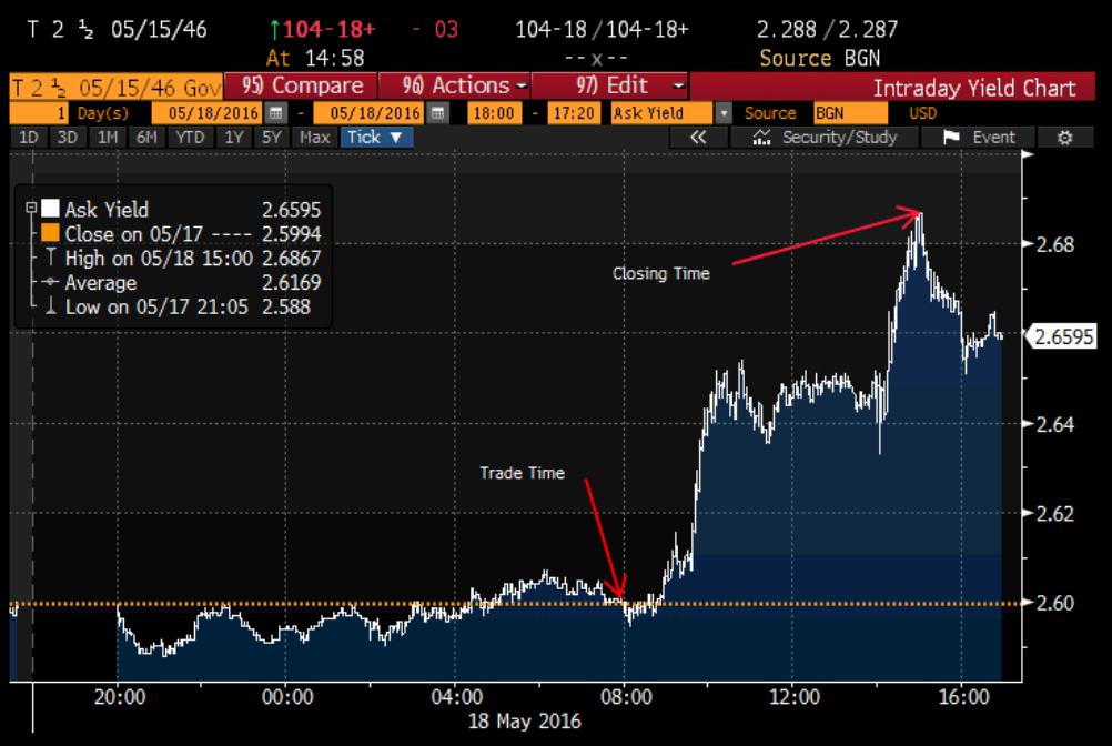
Figure 1: Intraday yield of 30-year Treasury on 5/18/16, showing rise of 9 bps
Given the rise in yields, the price of the corporate bond would have adjusted downward by -16.5 * 0.09 = -1.485%. Thus, the closing price would have to be 104.33. We make such an adjustment to the price of the bond as part of our process; most pricing services do not.
Figure 2 is a screenshot of the traded time of our corporate bond and Figure 3 is a table of its historical closing price, with the shaded cells corresponding to 5/18/16.
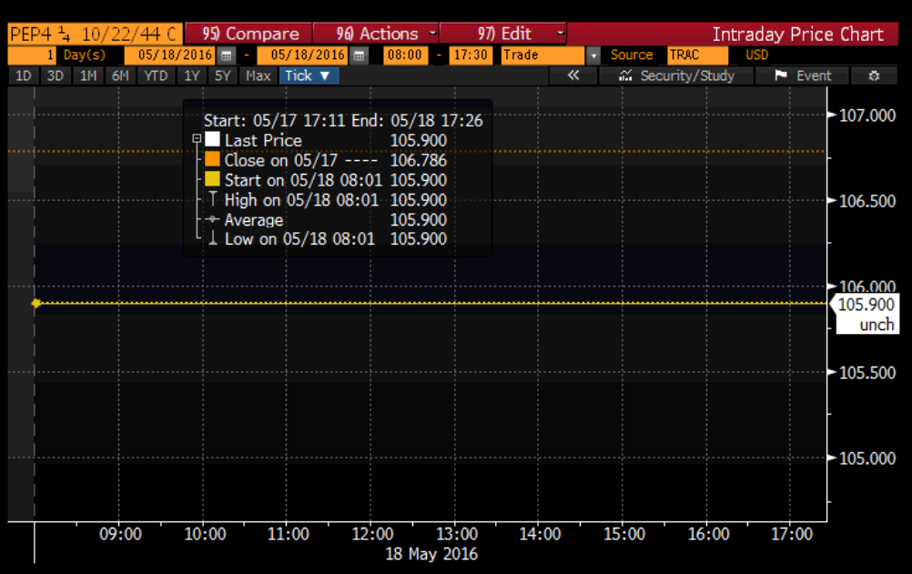
Figure 2: Intraday price of PEP 4.25% 10/22/44 – 5/18/16
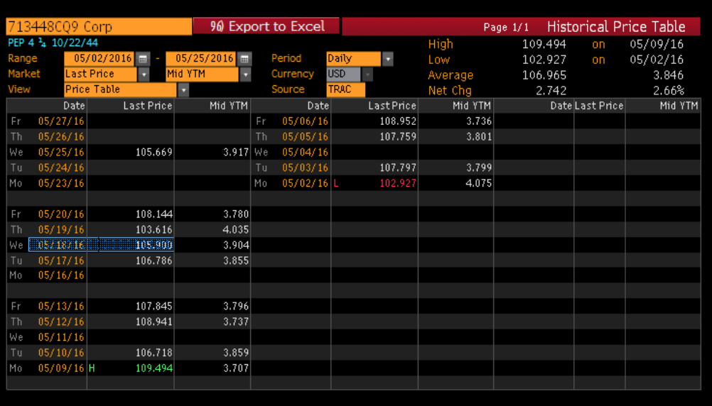
Figure 3: Historical price of PEP 4.25% 10/22/44 - 5/18/16
Trading in the US usually continues past the 3:00 PM cutoff time and due to the globalization of trading, many securities trade around the clock. We capture any other trading that takes place after 3:00 PM and use that for future analysis and for calculating the spreads of bonds that don’t trade every day.
Summary
Our pricing process involves the following steps:
- Obtain prices and perform intraday adjustments.
- Perform historical time series analysis of the price moves; bonds with suspicious prices are treated as if they had not been priced.
- Calculate the term structure of all rates and rescale them to correct for prior day’s bonds prices (see the Non-Callable Credit Bonds Section in the Appendix).
- Price unpriced securities.
- Calculate new term structure of all rates.
- Recalculate all durations, spreads, and call values, including bonds that were flagged in Step 2, using their quoted market prices.
- Perform time series and cross-sectional analysis as follows:
- Time series analysis on prices, similar to Step 2
- Time series analysis of spreads relative to the respective curves
- Cross-sectional analysis of yields and comparison with out-of-sample averages and standard deviations
- Analysis of the daily changes in the spread of bonds relative to the issuer’s curve
- Calculate new prices for flagged securities. A bad price is usually flagged by more than one of the four above methods.
- Repeat steps 5 and 6 with new prices.
It should be noted that a price may be flagged by one method but not by others. For example, if the price of a bond that has only three months to maturity changes by 0.25%, its spread changes by 100 bps, resulting in a flag in spread time series analysis but not in price analysis.
Our adjustment process employs a soft barrier methodology. For example, we don’t completely revise a price that is 3 sigma away from mean, but we leave a 2.99 sigma event unchanged. We use a continuous method of deriving new prices that is a function of the price deviation from mean. As such, the prices of all bonds are revised, even US treasuries. However, the revision for a treasury bond price can be in the 3rd or 4th decimal place, but the revision for a corporate bond price can be several points.
Appendix:
US Treasuries
US treasuries are the most liquid of all fixed-income instruments. Even though they trade primarily OTC, partly due to their size and partly due to the exchange-traded futures which closely track cash bonds, they tend to have a bid-ask spread of about one tick (1/32) for liquid securities and yield spread of about one basis point for most STRIPS. Figure A-1 shows the TSR for US treasuries.
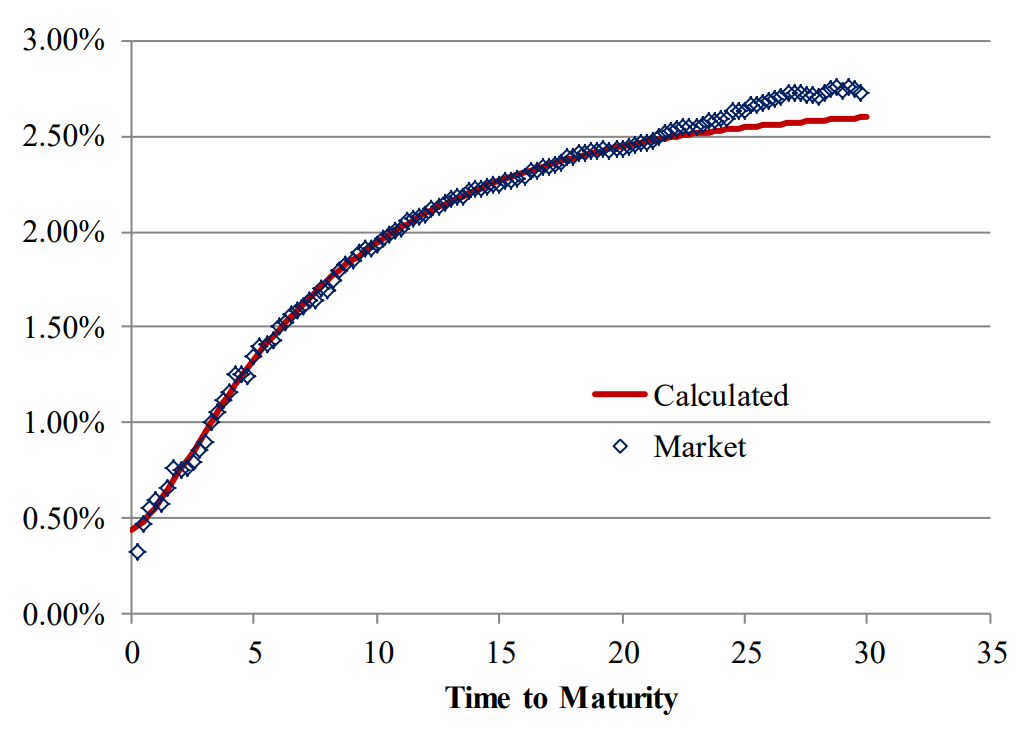
Figure A-1: Term Structure of Rates and Market Prices 2/12/2016
The calculated curve is the spot curve and is comparable to the treasury coupon STRIPS. The standard deviation of the difference between the calculated yield of treasury STRIPS and the market yield is less than one basis point up to a maturity of more than 20 years. The resulting pricing error if we use the curve for it is less than the traded bid-ask spread. Longer dated STRIPS have a positive spread to the curve, but the spread will not affect the pricing accuracy, as will be explained shortly.
Figures A-2 and A-3 show the time plot of the continuously compounded yield and spread relative to the TSR of the 20-year treasury respectively. The range of spread of the security relative to the curve is less than two basis points, even though this security was not used to calculate the curve. The daily variation of the spread is less than 0.25 basis points with a strong mean reversion tendency.
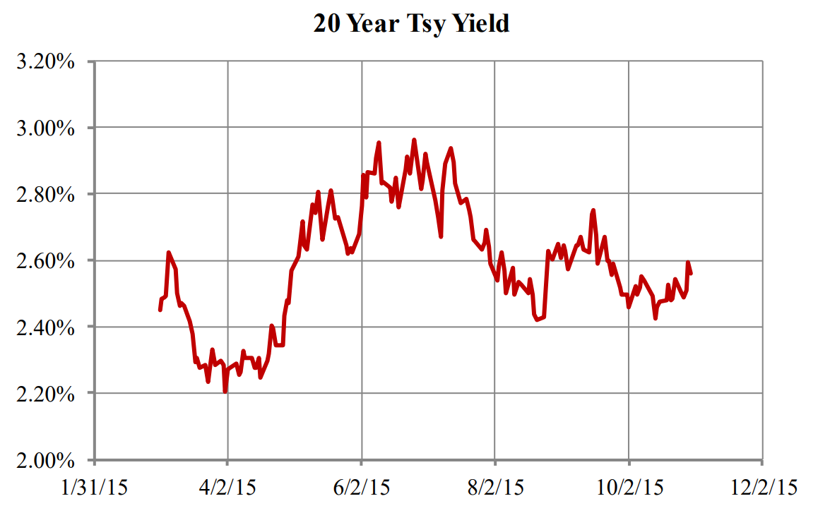
Figure A-2: Yield of 20-Year Treasury
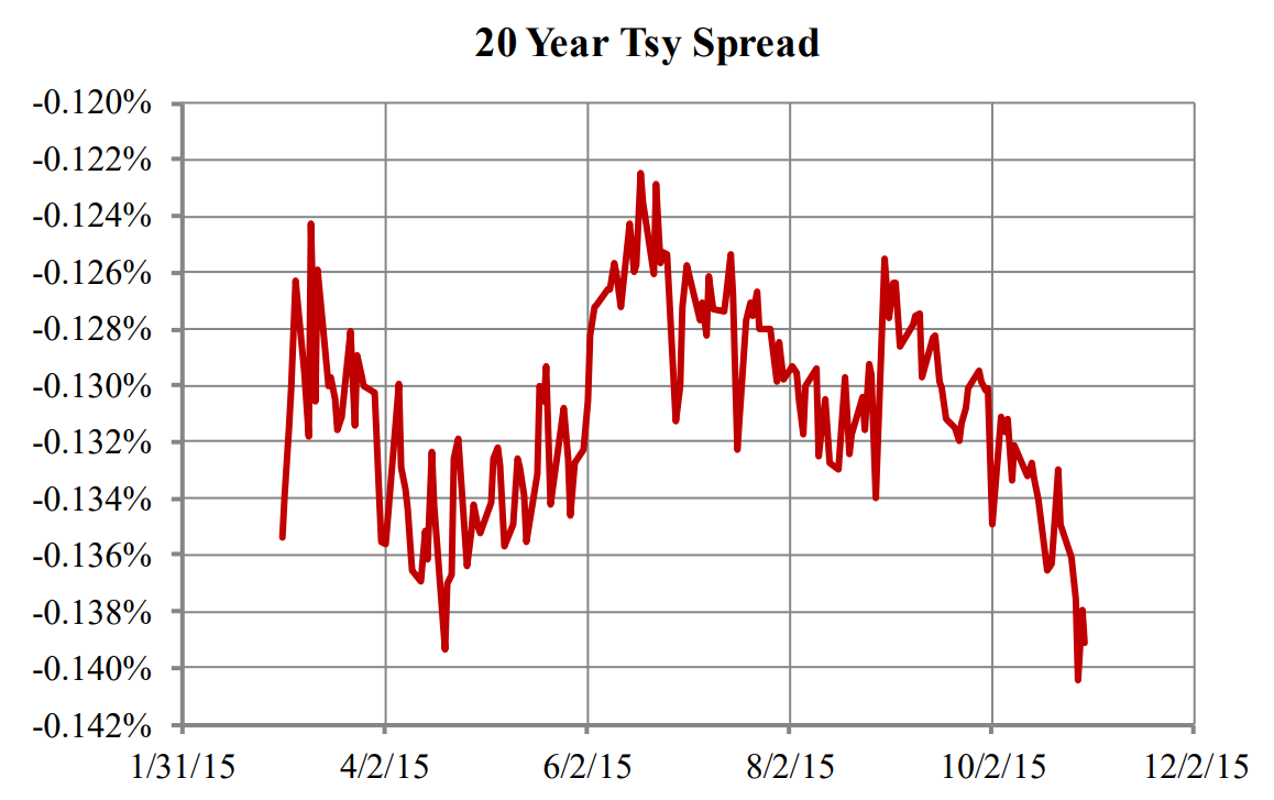
Figure A-3: Spread of the 20-Year Treasury Relative to the TSY
The stability of the spread of a security relative to its curve is the basis of our pricing methodology. The TSR is a representation of the entire market of an issuer. Most market participants are aware of the relative value of different securities, and if a security becomes too cheap or rich relative to its peers, traders take advantage of the pricing opportunity and bring the spread in line with the curve. Other factors such as liquidity, size of an issue, and coupon rate all contribute to the desirability or lack thereof of a security, and result in a market-consensus stable spread for a security. The spread can change from one day to the next, but its changes are generally smaller than transaction costs and are highly mean reverting.
Matrix pricing uses similar reasoning for pricing, but the pricing error tends to be about 50% higher than curve pricing, since the matrix or reference security is subject to price variation. Reference securities themselves tend to have higher spread volatility due to the liquidity premium at the time of issuance. Figure A-4 shows the spread of the 10-year treasury issued on 2/15/2015. The security had a spread of -14.5 bps at the time of issue and over the following six months the spread changed by 6 bps. Compare the range in Figure A-4 to Figure A-3.
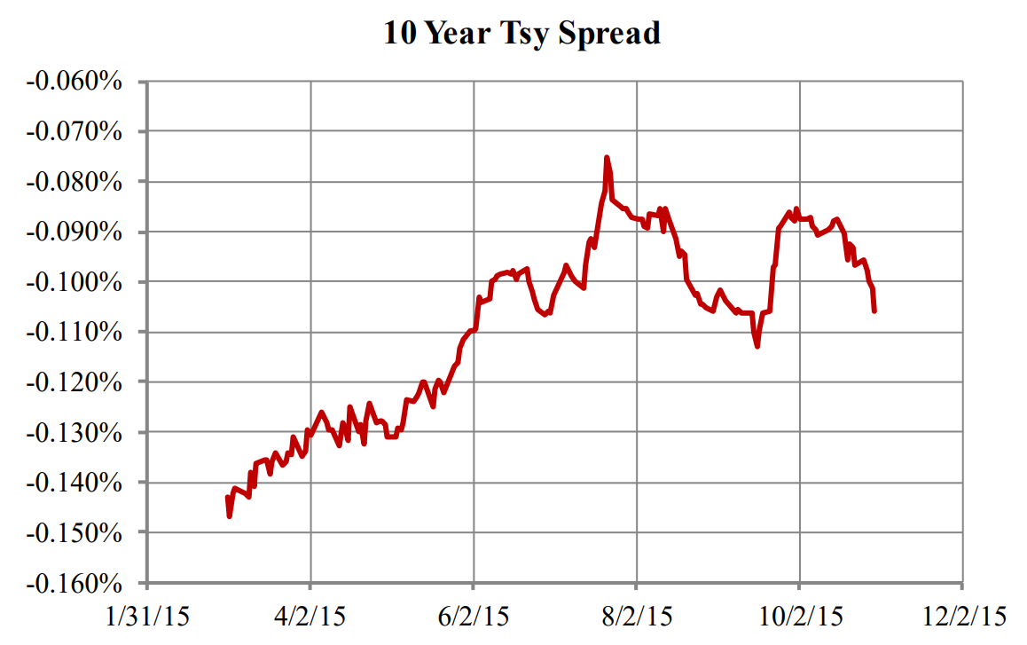
Figure A-4: Spread of the 10-Year Treasury Relative to the TSR
The spread volatility of reference or benchmark securities can result in a significantly larger pricing error at times of crisis when liquidity premium can be very volatile and large, such as the period post Lehman bankruptcy.
Global Treasuries
Most global government bonds have very good liquidity, and many are exchange-traded. We calculate a TSR for all global governments and real rates where the data is available. When an illiquid bond trades, we capture its spread relative to the respective curve and use that spread to price the security on other dates. If no spread is available, we assume that the spread is zero.
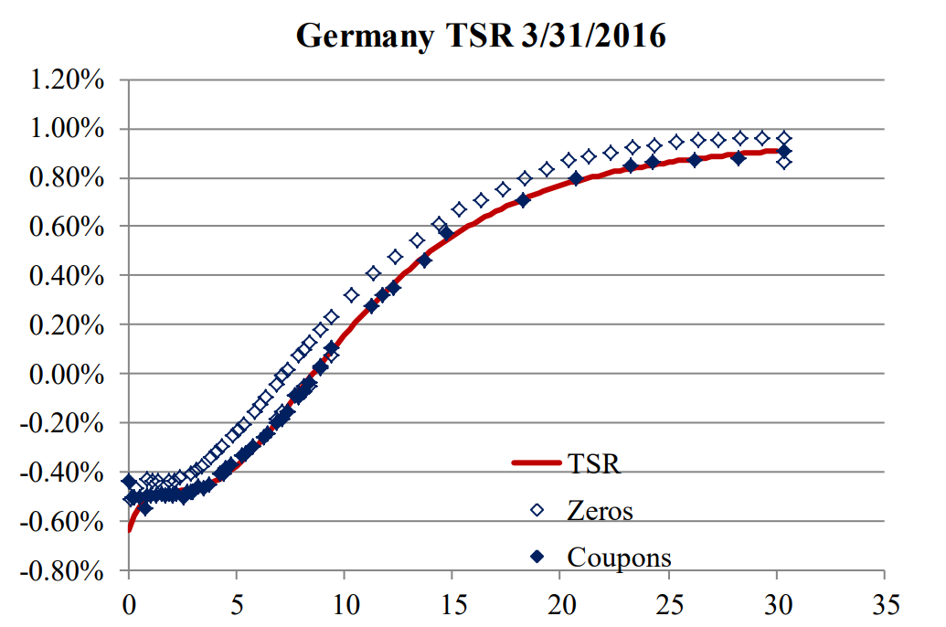
Figure A-5: German Government Curve and Traded Securities
Figure A-5 shows the TSR of German government bonds including zero-coupon bonds. For coupon bonds, we calculate their spread relative to the curve, and simply add that spread to the spot curve (TSR) for visual purposes. Solid diamonds represent the coupon bonds and were used to calculate the TSR. Blank diamonds are based on the market price of zero-coupon bonds. Here is a very good case of market segmentation; traders prefer coupon bonds and are willing to pay a yield premium of 15 bps over zero-coupon bonds. A portfolio manager can simply replicate a coupon bond by buying a stream of zero-coupon bonds. Had we built our TSR from zero-coupon bonds, coupon bonds would fall under the TSR. Table A-1 shows some of these bonds.
| Coupon | Maturity | Price | Spread |
|---|---|---|---|
| 0 | 2/15/23 | 100.29 | 0.153% |
| 0 | 5/15/23 | 100.06 | 0.158% |
| 0 | 8/15/23 | 99.88 | 0.155% |
| 1.5 | 2/15/23 | 111.84 | -0.008% |
| 1.5 | 5/15/23 | 112.12 | -0.015% |
| 2 | 8/15/23 | 116.07 | -0.016% |
Table A-1: German Government Bond Prices and Spreads
Figure A-5 shows the uniformity of the spread of bonds above the curve or right on it. The uniformity is also a sign of stability of the spread, and the spread can be used to price bonds that are not traded.
Non-Callable Credit Bonds
Our methodology for pricing corporate bonds and agencies is similar to that for pricing treasuries. However, the market depth (size and liquidity) and breadth (number of maturities) of corporate bonds is significantly lower than that of government bonds. Most corporate bonds have outstanding amounts of about $250 million or less. Assuming a very conservative average position size of $2.5 million for each fund manager, the number of holders for a $250 million issue will be about 100. If the average holding period is one year, the expected number of trades will be about twice a week. For this reason, many corporate bonds don’t trade every day, but still need to be priced daily for fund managers that have them in their portfolios.
Consider a 10-year credit security with a spread of 150 bps over the US treasury curve (Figure A-1). Now assume that the same issuer has a 20-year bond with a spread of 200 bps. From these two bonds we can estimate that if the issuer has a 5-year bond, its spread should be less than 150 basis points. We take this concept and develop a Term Structure of Credit Spread (TSCS) from the traded credit securities in the market. We use the five components of the TSR for calculating government curves, but we limit the number of components to three for credit securities. Even for agency bonds which can be more liquid than many government bonds, three components are sufficient.
Given the liquidity and breadth of agency bonds such as FNMA or FHLM, their credit spread can be fully explained by three components of our TSCS to an accuracy of about 2-3 bps.
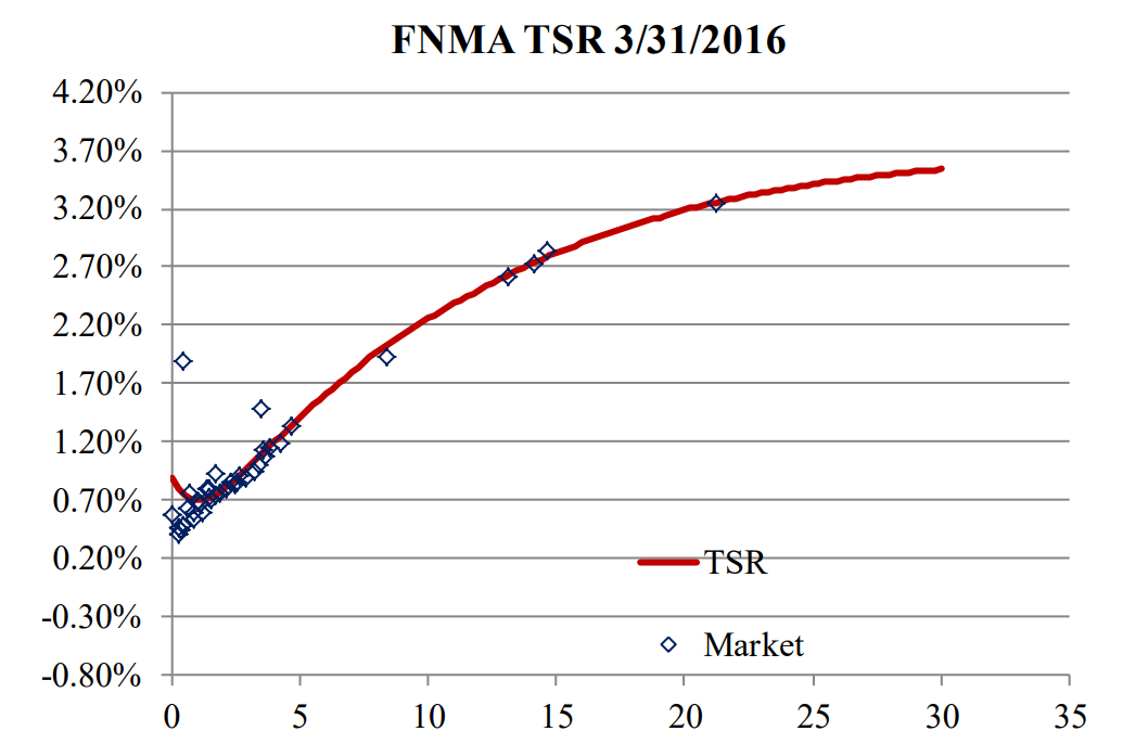
Figure A-6: FNMA Curve and Traded Securities Using Three Components
Now, consider a corporate issuer with ten outstanding bonds and suppose that only six of those bonds trade on a given day. We calculate a TSR for that issuer using six bonds and use a maximum of three components to price them. On the following day, if five bonds of the issuer trade, we will calculate a TSR for those five bonds. Now assume that only three of the five bonds traded on the previous day. We adjust the level of the TSR on the second day in such a way that the three bonds that traded on both days are on average correctly priced. This step is a critical component of our pricing methodology and ensures that the aggregate traded bonds (not individual reference securities) have market prices. Once we adjust the TSR, we can price the two bonds that were traded the day before from their spreads to the curve.
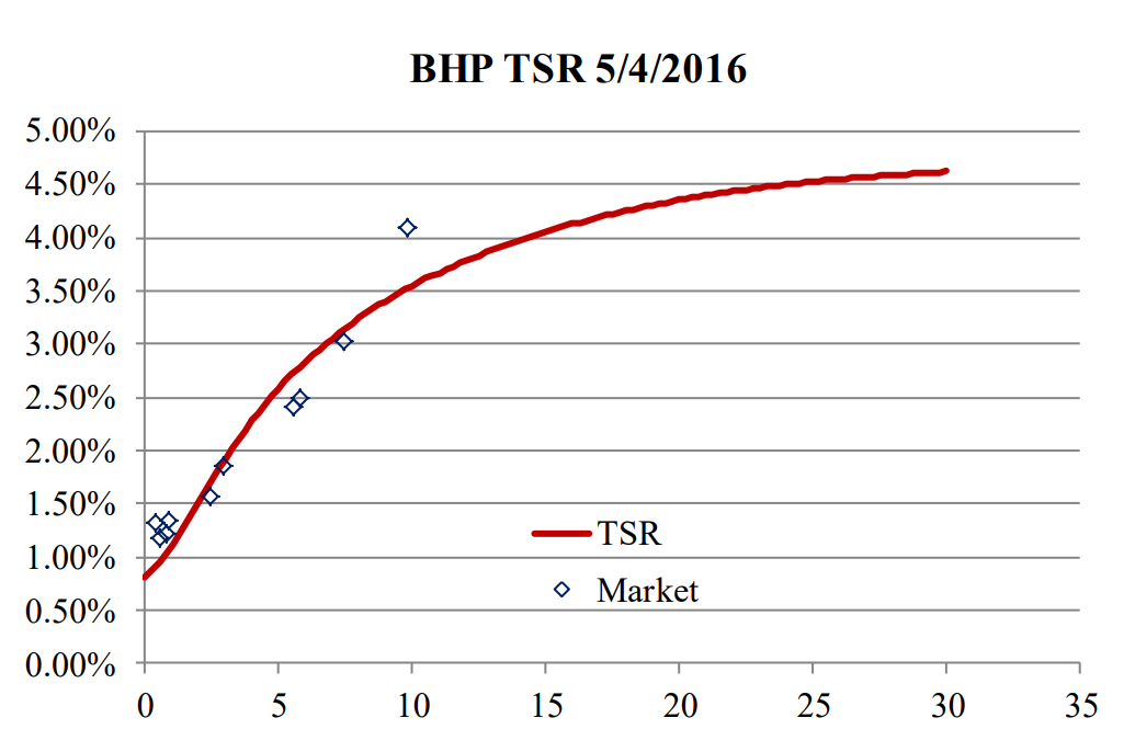
Figure A-7: BHP Curve and Traded Securities Using Three Components; 5/4/2016
Figure A-7 shows the TSR for BHP on 5/4/2016 along with traded bonds. The fit is not very good and one of the bonds with a maturity of 10 years has a spread to the curve of more than 50 bps.
On 5/5/2016 the bond with a maturity of 10 years did not trade, but two bonds with maturities of longer than 25 years traded. The calculated TSR for 5/5/2016 is shown in Figure A-8. The fit is significantly better than the previous day. We can speculate that the bond with a maturity of 10 years is an old legacy bond that was issued in 1996, is not liquid and has a large spread.
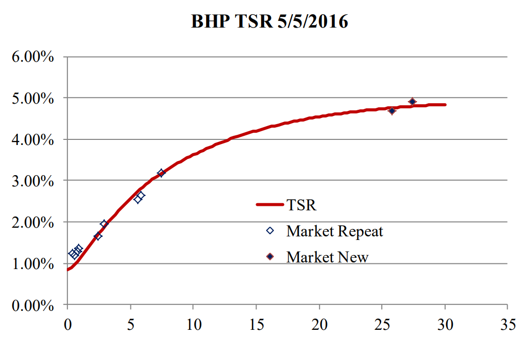
Figure A-8: BHP Curve and Traded Securities Using Three Components; 5/5/2016
The calculated TSR in Figure A-8 can’t be used for pricing. If we used the spreads that were calculated on 5/4/2016 for traded securities and applied them to the curve in Figure A-8, the resulting prices would be different from the market prices on 5/5/2016. There is no curve that can correctly replicate the price of all bonds that traded the previous day, but we can calculate a shifted curve that would correctly price the aggregate of all the bonds that traded on both days. The adjusted curve is shown in Figure A-9.
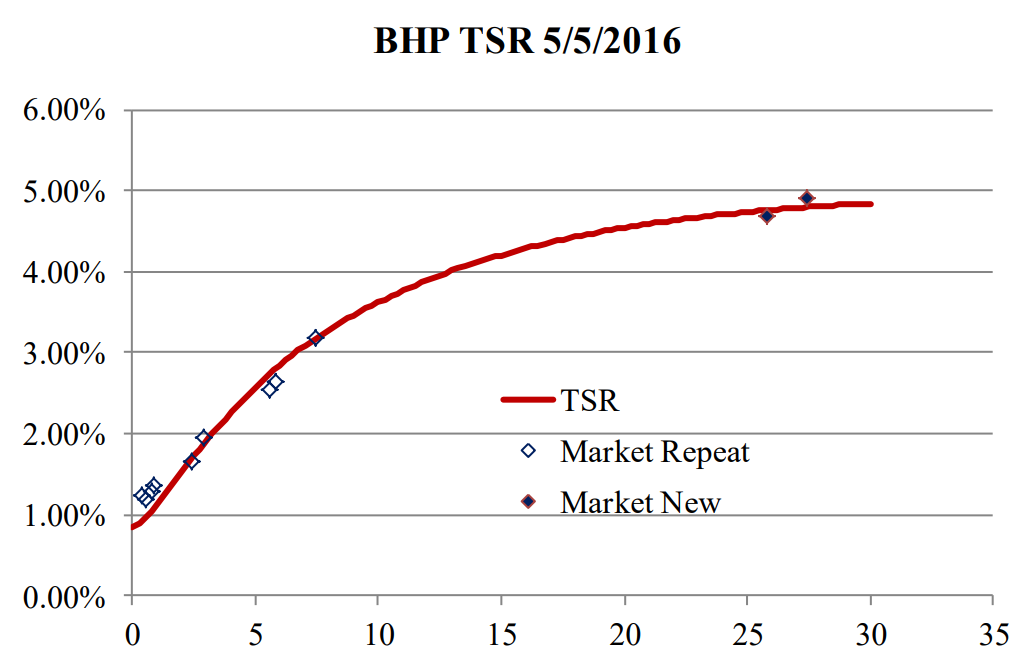
Figure A-9: BHP Adjusted Curve and Traded Securities Using Three Components; 5/5/2016
Comparing Figures A-9 and A-7, we can see that securities with a maturity of between 5 and 10 years are slightly below the curve and are positioned similarly relative to the curves. However, the same bonds are positioned closer to the curve in Figure A-8.
We can use the curve in Figure A-9 to price the bond with a maturity of 10 years in Figure A7 that was not priced on 5/5/2016 after performing time series analysis—a subject that will be discussed in the following sections.
There are many corporate, emerging markets, or sovereign securities that are not priced by most pricing sources. We can price those securities from their curves. Figure A-10 shows the daily price of one such security. Figure A-11 shows the intraday pricing of the same security. It is interesting to note that even though during the day it trades at various prices, it closes at a price of 132.
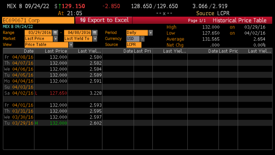
Figure A-10: Historical price of a Mexican bond
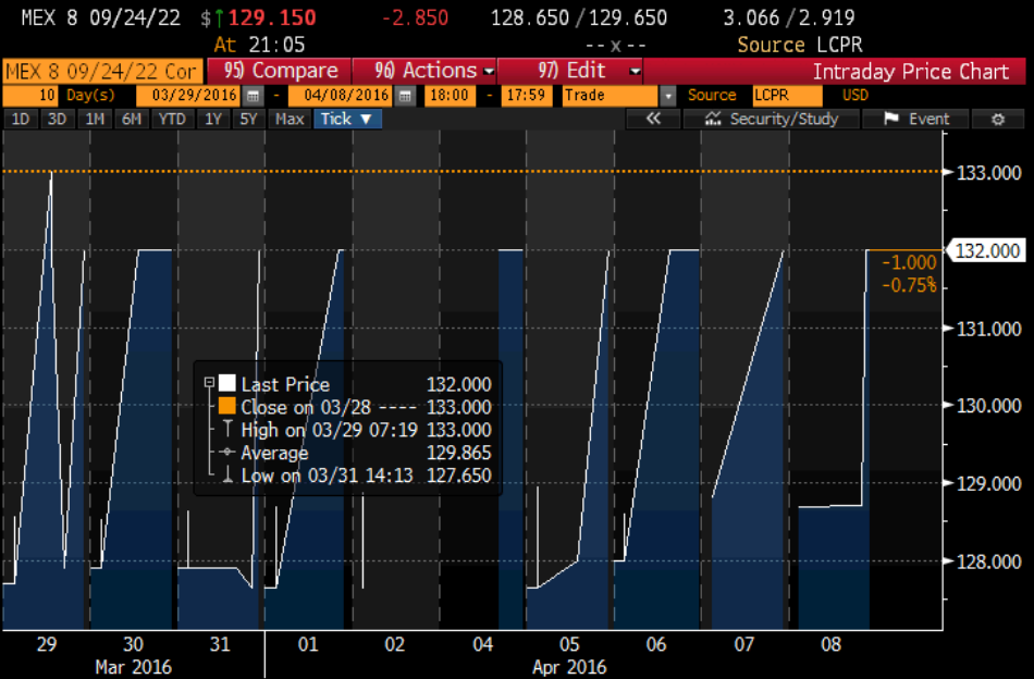
Figure A-11: Intraday price of Mexican bond
Callable Bonds
The valuation of the call value of a callable bond is a very complex business. Since nearly all callable bonds have a call option that can be exercised at any time after the first call date, their valuation is completely different from European options which can be exercised only on a single date. Even major pricing service providers can sometimes be off in the calculation of American option values by more than a factor of 2. We argue that our model, as described in The Advanced Fixed Income and Derivatives Management Guide, is virtually the only model that is not only accurate but practical.
We calculate the Term Structure of Volatility (TSV) for countries where the data is available. Callable agency bonds are priced by assuming a beta and correlation of one with the TSV. This is an accurate assumption, since agencies often issue floating rate bonds with a spread of plus or minus a few basis points to the RFR.
For corporate bonds, we use a correlation of 0.5 and a spread beta of about 0.8 to estimate the value of the call option. Once the option value is calculated, we calculate the implied yield volatility that would price that option accurately and use the same volatility to calculate the value of the option on a following day if the bond’s price needs to be calculated. The reason for this approach is that traded volatilities can sometimes have pricing errors. For example, in one instance the 2-year forward volatility of a 3-year bond, which was 50% on one day, increased to 59% the following day. The call value of an out-of-money 5-year bond that was callable in two years increased from two to about five due to the change in volatility. This would imply a three-point drop in the value of the bond; however, the change in price was significantly below that. For this reason, the call value is calculated based on the implied volatility of the previous day.
Once we calculate the call value of a callable bond, we price an otherwise non-callable bond from its spread to curve and subtract the call value to calculate the price of the callable bond.
We argue that without good derivatives capabilities, pricing services cannot accurately price callable securities. Without calculating the call value, there is no sound way to model the price of a callable bond that has not traded. Matrix pricing or interpolation can’t be used for pricing callable bonds, especially when the bond is trading close to the call price. Hence, there are many callable bonds that are either not priced or not priced correctly. Figure A-12 is the price table of a zero-coupon bond that is not priced by a major pricing service. This bond is callable by yield. The price table shows that for an entire year, the bond was priced at 100.
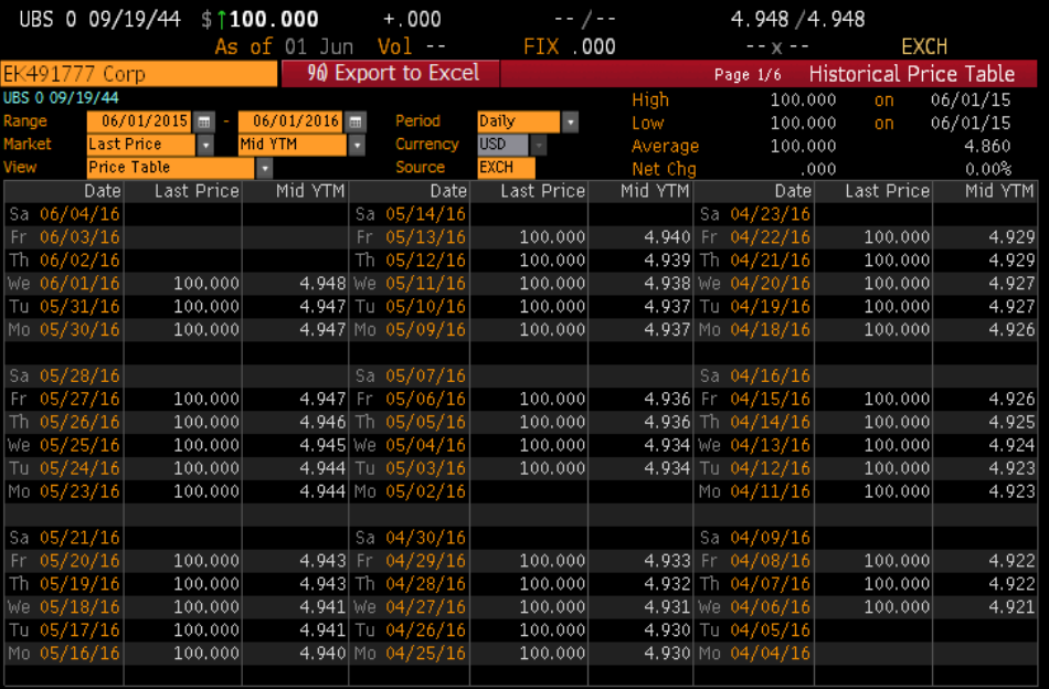
Figure A-12: Zero-Coupon Callable Bond; high and low prices are 100 for the year
We price such bonds by calculating the call value and subtracting it from the present value of the security, assuming that it is not callable.
Bonds Without a TSR
There are many issuers that have only one or two outstanding bonds with a given rating. For these securities, a TSR can’t be calculated. We price these bonds based on generic TSRs that we produce from the aggregate of all TSRs in a given currency. We segregate about 600-800 TSRs that we calculate daily for US corporates into 16 tranches, based on their yield levels, which we assign internal ratings from AA+ to CCC+ through a rigorous process that eliminates suspect TSRs. The TSR for each tranche will be the average of about 30 corporate TSRs; they represent our own internal rating based on market yields. We believe this is a better method of defining ratings than using rating agency values, since the markets quite often anticipate a rating change and price bonds accordingly. Moreover, bonds that have no ratings will be easily classified into one of our tranches based on their yield or spread and maturity.
Every bond in the market will be assigned a rating, and its spread relative to that rating is calculated every day. If the bonds of an issuer are not traded at all on a given day, we use our internal rating of that issuer to estimate its price change. This is a very safe method for pricing bonds that have not traded. If a credit event occurs, the bonds will trade actively, reflecting updated market conditions, and their prices will adjust naturally to incorporate the impact of the event, making it unnecessary to rely on estimation or assumptions.
For example, suppose that an issuer has two bonds, X and Y, with maturities of 5 and 20 years and spreads of 20 and 25 bps relative to their internal BBB TSR on a given day. If on the following day, bond X trades with a spread of 16 bps relative to the generic BBB, we then estimate that the spread of Y has contracted by 4 bps relative to the generic BBB, and thus we price it accordingly.
Note that the change in spread is relative to the curve, which itself is subject to a change in shape. For example, on a day that payroll data is weak, the yield curve can steepen and the yield difference between 5- and 20-year maturities increases by 10 bps. In our example, even though the yield of Y has contracted by 4 bps, the curve has steepened by 10 bps, resulting in a net increase in yield of Y relative to X of 10 bps. For a bond with a 20-year maturity and 12-year duration, the price impact would be 1.2%. Matrix pricing would not capture the 10-basis point change in the shape of the curve.
If a traded bond has a very short maturity, its yield adjustment can be very large and unrealistic; we ignore the yield change of bonds with a maturity of less than one year. For example, if the price of a bond that matures in two months changes by a bid-ask amount of 0.25, the implied yield shift will be 150 bps. Such a yield shift is not reasonable and can distort the price of long-dated bonds by several points.
Likewise, we assign an internal TSR to all callable bonds. If the issuer of a callable bond has other bonds that are not callable, we use their generic TSR for valuation of the callable bond. If there are no non-callable bonds, we assign a generic TSR by iteration. We estimate the yield to worst and use that as a starting point to assign a generic TSR. We then calculate the option value and estimate the yield of a non-callable security. From that yield, we assign a new TSR and repeat this process.
Swaps and the RFR
We calculate a TSR for the RFR and swaps for more than 30 countries. Our TSR for developed markets is very accurate, and within 1-2 bps of the actual traded market. Through the Adjustment Table (see AFIDMG) we replicate the market-traded prices of all swaps and can use our TSR to price off-the-run swaps. Our model uses the smooth TSR instead of interpolation and we believe it to be the most accurate of all practical models in the market:
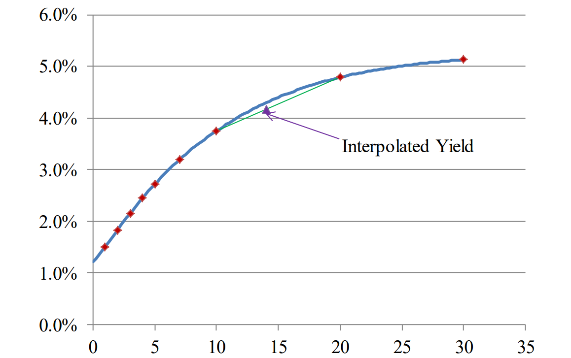
Figure A-13: Zero-Coupon Swap Curve
In Figure A-13, the interpolated yield would be off by about 13 basis points from the curve resulting in a pricing error of about 1.35%.
Bond Options and Swaptions
Bond options are completely different from equity options. Unlike equities, bond prices have a maximum value. As the approach maturity, bond prices converge towards par, causing option values to fall. Additionally, a forward bond has different durations and risks compared to a spot bond.
European bond options can only be exercised at expiration, while American bond options can be exercised from a start date through an expiration date, and they can be continuous or discrete (coupon payment dates). Callable bonds are usually like American bond options.
The arbitrage-free requirement imposes a very stringent constraint on the possible distribution of all outcomes, which ensures that the price of a call and a put are equal at option expiration for an at-the-money option. This is called call-put parity. However, this is true only at the expiration date, and for the present time the call-put parity is not applicable to fixed-income options. The money-forward call must be discounted at a lower average rate than a forward put, since the path of rates that will lead to a call imply lower forward discount rates—while the opposite is true for a put option.
The most popular method of pricing the value of bond options is Black-76 which assumes that interest rate volatility is similar to equity volatility. Since price-yield relationship is not linear, Black-76 is not strictly arbitrage-free. For short-dated options, the pricing error is very small, but for long-dated options and callable bonds, Black-76 is not accurate. Additionally, Black-76 assumes a constant volatility at all forward rates and there is no mechanism to discount call options at a lower rate than put options. Since 2008, the 1-year volatility of short rates has been more than double the volatility of long rates, thus the assumption of constant yield volatility has not been borne out by the markets.
Our proprietary method, in contrast, has the accuracy of a closed form solutions for bond options, if such a one existed. Unlike Black-76, we impose the arbitrage-free requirement on the price of the forward paths of interest rates, and at every future exercise point we use a discount function that reflects the average path of interest rates to get to that point. Our volatility surface perfectly matches all volatilities at all forward rates exactly (with the market traded volatility).
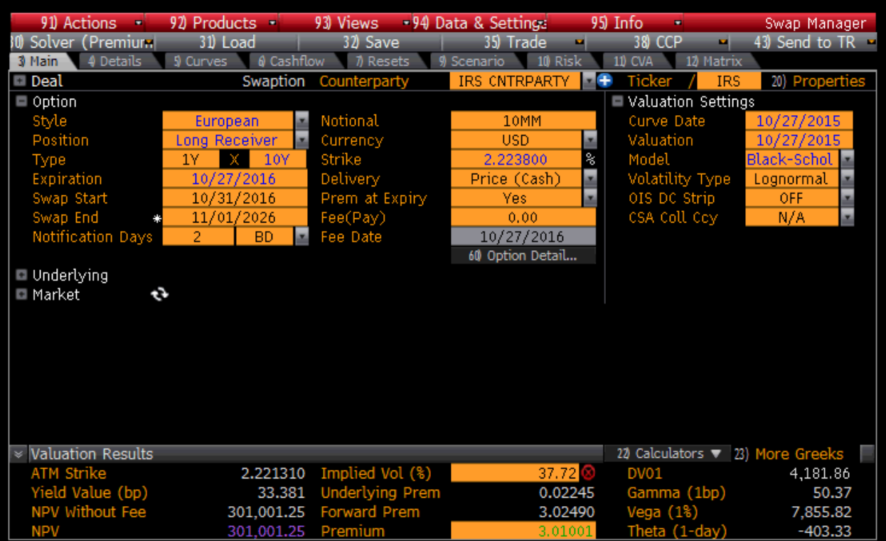
Figure A-14: 1 X10 European call swaption price from a major pricing service – 10/27/2015
Figure A-14 shows the calculated price of a European call swaption on 10/27/2015, for a 1-year x 10-year to be 3.01. The Black-76 model yields a value of 2.95 and our model is very close at 2.933. The price from the major pricing service appears to be off, even though forward rates are the same. For longer-dated options, where convexity becomes significant, the pricing error of the Black-76 model is much higher. For a 5-year by 20-year forward call option Black-76 produces a price of 9.95 while our model is 9.53.
For American options, the universally accepted method of calculation is building a binomial tree. However, binomial tree models—and Monte Carlo models—converge very slowly with the square root of the number of steps and are not practical solutions for pricing bond options. Moreover, binomial models have few nodes for early exercise, leading to relatively large pricing errors.
Again, our proprietary method achieves superior results, having the precision of closed-form solutions for bond options, if such solutions were available. At each future exercise point, we apply a discount function that accounts for the average path of interest rates leading to that point. Additionally, our volatility surface aligns perfectly with market-traded volatilities, matching all forward rate volatilities exactly.
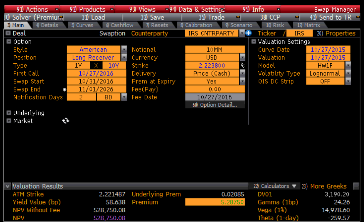
Figure A-15: 1 X 10 American call swaption price from a major pricing service – 10/27/2015
Figure A-15 shows the calculated price of an American call swaption for the swap in Figure A-14. The calculated premium by the major pricing service is off by about 60%. Because the options are for forward at the money and the yield curve is steep, the forward implied coupon would be higher than the coupon of a 10-year swap at the present. If the American call option is exercised immediately, the premium would be worth 1.73. However, given that the option premium is much higher, it does not make sense to exercise the option immediately. Suppose that there is 50% probability to exercise the option, and we assume that there is a constant probability that the option will be exercised any time through the expiration. In this, on average, the option will be exercised in six months, and we will realize about 1.73 extra than we would with a European option with a 50% probability for six months, i.e., 1.73/2 × 0.5 = 0.43. Thus, the premium should be worth about 0.43 over a European option. However, this amount is overstated, since the likelihood of an exercise in the first month is significantly less than the likelihood of an exercise in the last month. If we assume that the probability of exercise is not a constant, but rather is proportional to time, we can estimate the premium should be about 1.73/6 = 0.29 over European. Our model provides a premium of 0.32 more for the American option vs. European option.
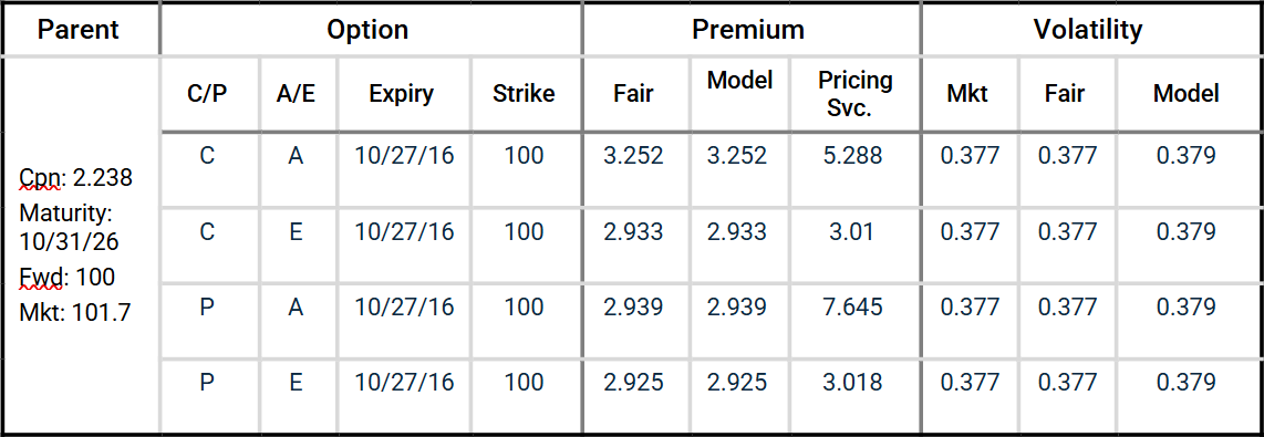
Table A-2: Option Premiums: Our calculations compared to a major pricing service’s.
The major pricing service’s premium of the American put option appears significantly misaligned, considering that—given the steep yield curve—the early exercise of the option is not likely, and thus the prices of the American and European puts should be very close.
Corporate Bond Options and Callable Bonds
We have developed what is likely the only process for pricing a credit security’s fixed-rate and floating-rate options consistently. Corporate bond options require a correlation model and spread beta, which can be obtained from historical values. Outside of the RFR (swap) arbitrage-free requirement, a second dimension must address the arbitrage-free forward distribution of credit rates consistent with the beta and correlation. This additional dimension requires a three-dimensional swap-credit-time volatility surface. Our process achieves this, enabling us to price credit options accurately and consistently.
For example, for a corporate issuer with both fixed and floating-rate callable bonds, we can price both options by using the same beta and correlation coefficient arbitrage-free and do so in a uniquely practicable way. Monte Carlo simulations in three dimensions, in contrast, converge much too slowly to be of practical use for pricing corporate options. Our model, therefore, is the most practical method for pricing an issuer’s floating and fixed-rate bonds consistently.
Other Options and Currencies
We price all currencies and currency forwards by building a TSR specifically for currency forwards. From this TSR we can calculate the forward price of any currency relative to any other currency.
Options on currencies are generally the most diverse of all options, and many exotic options trade primarily for currencies. We price exotic options using closed-form solutions and we can—relatively quickly—model some of the most complex options on currencies and other assets. For example, we can price a long-dated option on a global stock index future, provided that EURUSD is below or above some level. Such an option is called a correlation option. The following list provides some of the options that we can price:
- Barrier Options
- Single Barrier Options
- Up and in call or put
- Up and out call or put
- Down and in call or put
- Down and out call or put
- Double Barrier
- Touch and in call or put
- Touch and out call or put
- Partial Time Barrier Options
- Early Monitoring
- Up and in call or put
- Up and out call or put
- Down and in call or put
- Down and out call or put
- Late Monitoring
- Up and in call or put
- Up and out call or put
- Down and in call or put
- Down and out call or put
- Look Options
- Floating Strike Look Options
- At expiration, the option holder has the right to exercise it at the extreme price that it traded during its life.
- Since the option is almost always exercised, the premium is very high.
- The strike price can be adjusted by a factor (f>=1 for calls, f<=1 for puts).
- The monitoring period can be adjusted to make the option partial time floating strike look.
- Partial Time Look Options
- The holder has the right to exercise the option at the highest value during the monitoring period.
- Partial Time Look Barrier Options
- If the barrier is not hit in the first monitoring period, a floating strike look option is issued.
- Other Exotic Options
- Soft Barrier Options
- A soft barrier option is partially knocked in or out depending on how much its price penetrates the gap between two barriers.
- There can be up or down and in and out for calls and puts.
- Digital (Binary) Barrier Options
- Digital options pay a fixed amount if the option at expiration is in the money or nothing at all.
- There are sixteen option combinations (call/put, in/out, up/down, asset/cash).
- There are eight combinations for knock-ins (up/down, asset/cash, when hit/expiry).
- There are four combinations for knock-outs that are both put and call.